mirna_pipeline

Analysis pipeline for “A comprehensive framework for analysis of microRNA sequencing data in metastatic colorectal cancer”
A reproducible analysis pipeline for the manuscript “A microRNA Signature of Metastatic Colorectal Cancer” by Høye et al. Integrates both public repositories and own smallRNA-seq data. Quality control with the expertly developed miRTrace quality control and contamination detection pipeline. Data processing and read alignment with miRge3.0, using our curated database MirGeneDB as a high quality miRNA gene reference. miRge3.0 count matrixes used for downstream analysis, including data exploration with UMAP, differential expression analysis with DESeq2 and inference of bulk tissue cell composition with known cell marker miRNA.>
References:
miRTrace Genome Biology (2018).
Kang W; Eldfjell Y; Fromm B; Estivill X; Biryukova I; Friedländer MR, 2018. miRTrace reveals the organismal origins of microRNA sequencing data. Genome Biol 19(1):213
miRge3.0 NAR Genomics and Bioinformatics (2021).
Arun H Patil, Marc K Halushka, miRge3.0: a comprehensive microRNA and tRF sequencing analysis pipeline, NAR Genomics and Bioinformatics, Volume 3, Issue 3, September 2021, lqab068, https://doi.org/10.1093/nargab/lqab068
Set up singularity container
# on a host with singularity installed, first clone the repository
git clone https://github.com/eirikhoye/mirna_pipeline
cd mirna_pipeline/

# Configure miRTrace container
sudo singularity build singularity/miRTrace.simg singularity/miRTrace.recipe

# Alternatively, install miRTrace by following instructions here:
https://github.com/friedlanderlab/mirtrace

# Configure miRge3.0 container
sudo singularity build singularity/mirge3.simg singularity/mirge3.recipe

# Alternatively, install miRge3.0 by reading instructions here for relevant OS:
https://mirge3.readthedocs.io/en/latest/installation.html
# and make sure dependencies are installed (python=3.7 and r) and bowtie, samtools and RNAfold
Usage
# running miRTrace singularity container
dt=`date '+%d%m%Y_%H%M%S'` # date time variable for output dir

sudo singularity exec --bind /path/to/project_folder_on_host:/mnt /path/to/miRTrace.simg mirtrace qc \
           --species hsa \
           --custom-db-folder /mnt/custom_databases/ \
           --config /mnt/config \
           -o /mnt/mirtrace_out/"$dt"

# running miRge3.0
sudo singularity exec --bind /path/to/project_folder_on_host:/mnt /path/to/mirge3.simg \
          miRge3.0 -s /mnt/filepaths.txt \
          -lib /mnt/miRge3_Lib \
          -on human \
          -db mirgenedb \
          -o /mnt/mirge_output \
          -tcf \
          -cpu 4 \
          -a illumina
Note, in order to work with your data in a singularity container you must mount the directory it is stored in (here called “project_folder_on_host”) on your host, on to a path inside the singularity container, here /mnt, with the syntax: /path/to/host_dir:/path/to/singularity_dir/. This way we can run singularity on files stored on our system. See https://sylabs.io/guides/3.0/user-guide/bind_paths_and_mounts.html for details.
Tutorial
Lets give an example using the FASTQ files in fastq_toy directory, using this study desgin:

Some toy fastq files as well as the singularity containers can be downloaded from this link: https://drive.google.com/drive/folders/1u-9NQ5rB9rbB_hzTWpNL8n1S2YXGyX6M?usp=sharing
First things first, lets do QC on these samples with miRTrace! miRTrace takes raw FASTQ files as input and outputs nicely formatted QC reports, and will also assess potential contamination.
miRTrace also requires a config .csv file with paths, name and library adapter sequence, of the format:
/mnt/fastq_toy/mLi_1.fq,mLi_1,TGGAATTC
/mnt/fastq_toy/mLi_2.fq,mLi_2,TGGAATTC
/mnt/fastq_toy/mLi_3.fq,mLi_3,TGGAATTC
/mnt/fastq_toy/mLu_1.fq,mLu_1,TGGAATTC
/mnt/fastq_toy/mLu_2.fq,mLu_2,TGGAATTC
/mnt/fastq_toy/mLu_3.fq,mLu_3,TGGAATTC
/mnt/fastq_toy/nCR_1.fq,nCR_1,TGGAATTC
/mnt/fastq_toy/nCR_2.fq,nCR_2,TGGAATTC
/mnt/fastq_toy/nCR_3.fq,nCR_3,TGGAATTC
/mnt/fastq_toy/nLi_1.fq,nLi_1,TGGAATTC
/mnt/fastq_toy/nLi_2.fq,nLi_2,TGGAATTC
/mnt/fastq_toy/nLi_3.fq,nLi_3,TGGAATTC
/mnt/fastq_toy/nLu_1.fq,nLu_1,TGGAATTC
/mnt/fastq_toy/nLu_2.fq,nLu_2,TGGAATTC
/mnt/fastq_toy/nLu_3.fq,nLu_3,TGGAATTC
/mnt/fastq_toy/pCRC_1.fq,pCRC_1,TGGAATTC
/mnt/fastq_toy/pCRC_2.fq,pCRC_2,TGGAATTC
/mnt/fastq_toy/pCRC_3.fq,pCRC_3,TGGAATTC
/mnt/fastq_toy/contaminated_1.fq,contaminated_1,CGCCTTGGCCGTA
/mnt/fastq_toy/contaminated_2.fq,contaminated_2,CGCCTTGGCCGTA
/mnt/fastq_toy/contaminated_3.fq,contaminated_3,CGCCTTGGCCGTA
/mnt/fastq_toy/read_len_1.fq,read_len_1,TCGTATGC
/mnt/fastq_toy/read_len_2.fq,read_len_2,TCGTATGC
/mnt/fastq_toy/read_len_3.fq,read_len_3,TCGTATGC

# note we set /mnt as prefix to path, because we defined our project folder as /mnt
Now lets run miRTrace from the singularity container
# First define some convenience variables
export PROJECT="/path/to/mirna_pipeline" # set to wherever you cloned the github mirna_pipeline directory
dt=`date '+%d%m%Y_%H%M%S'`               # date time variable, remember to reset before each run!
mkdir $PROJECT/mirtrace_out

# run miRTrace with
sudo singularity exec --bind $PROJECT:/mnt $PROJECT/singularity/miRTrace.simg mirtrace qc \
        --species hsa \
        --custom-db-folder /mnt/custom_databases/ \
        --config /mnt/config \
        -o /mnt/mirtrace_out/"$dt"
Now, in the $PROJECT/mirtrace_out directory, we will find a directory named with the date_time of this run. This directory contains Quality Control reports for the FASTQ files, both as .csv files and a nicely formatted .html file. Lets go through the content of this file now:
PHRED Scores
First lets look at the PHRED scores. A PHRED score is the likelihood that a nucleotide was called correctly, the higher the score, the more confident the nucleotide is correct. miRTrace flags a dataset if greater than 50 % of its nucleotides have a Phred score >= 30.

In this plot, all datasets but one, read_len_1, passed the Phred QC test.
Read Length Distribution
miRNA genes are 22 nt in length on average. The read length distribution in a smallRNA-seq datasets should be around 22 nt. If a large proportion of reads are outside this distribution, it is a good sign of issues during library preparation. miRTrace flags reads where less than 25 % of reads are in the correct range.

In this plot, the three rightmost datasets, read_len_1, read_len_2 and read_len_3, have reads in the incorrect range, and should therefore be excluded from the analysis.
Quality Control Statistics
miRTrace discards reads where there was no adapter detected or the length was less than 18 nt. A dataset is flagged if less than 25 % of reads pass these criteria.
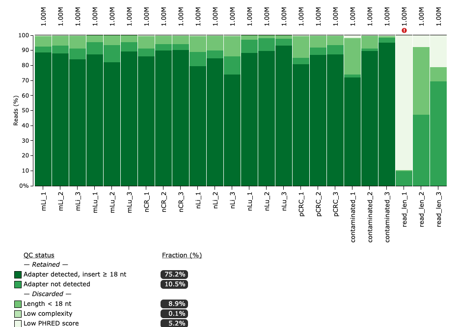
Again, we see that the three rightmost datasets, read_len_1, read_len_2 and read_len_3, had poor QC stats.
RNA Type
It is of course important that the dataset actually contains miRNAs. A low proportion of miRNAs in the dataset could be an indication of issues during library preparation, however this is also dependent on the type of biological sample being studied.

As expected, the three rightmost datasets contained no miRNA reads.
Number of unique miRNA genes detected
The number of miRNA genes that have been detected in the sample. Important to note here that MirGeneDB is used here, rather than miRBase with 1881 human miRNA genes, the majority of which have been shown to be false annotations.
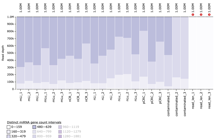
Now we also notice the datasets contaminated_2 and contaminated_3 have fewer number of detected miRNA genes than expected! As they passed all preceeding QC steps, this is unexpected!
Contamination
Lastly, miRTrace allows the detection of contaminants in miRNA datasets. Contaminated datasets are a strong indication of poor laboratory protocols, or mixup of barcodes when pooling samples on a flow cell. If a study has datasets with contaminants, one should concider not including those datasets in the analysis.
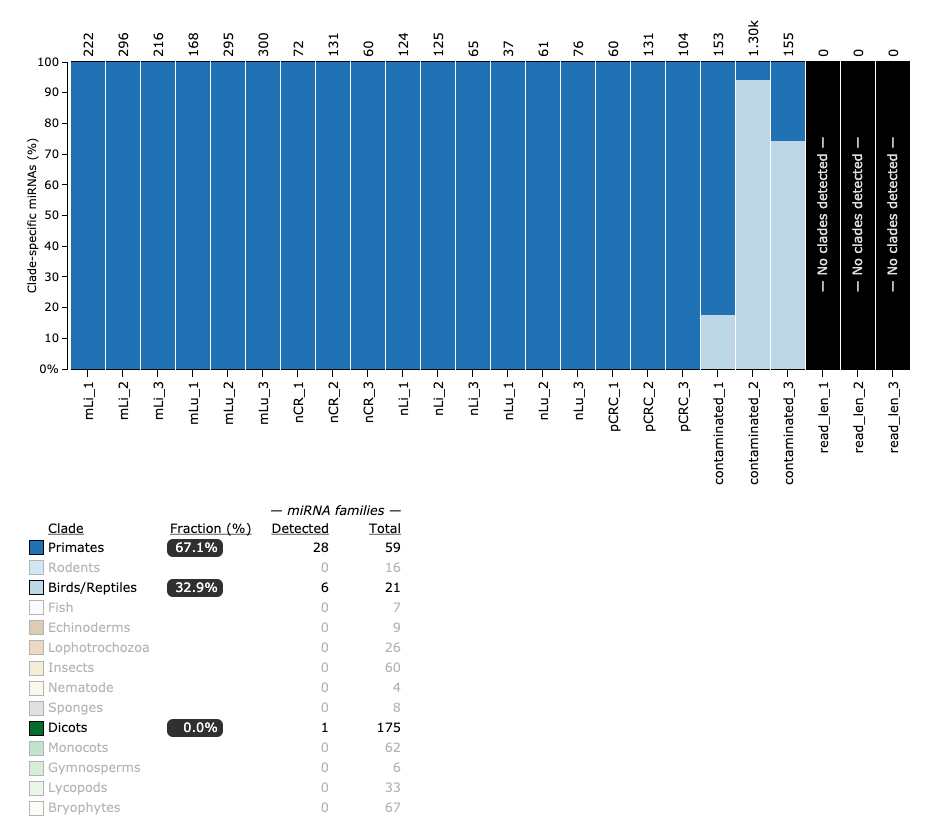
Now we see the cause of the lower number of detected miRNA genes in contaminated_2 and contaminated_3! The majority of miRNAs in these datasets are from bird/reptile clades! Needless to say, these datasets should also not be included in further analysis.
miRge3.0
Now that we have run our datasets through QA, its time to align those that passed to MirGeneDB2.0. To do this, we will use miRge3.0, a state of the art read aligner that is designed specifically for miRNA datasets. miRge3.0 has many advanced features, including detecting A to I editing events, discovery of novel miRNAs, and much more. For further details, see https://mirge3.readthedocs.io/en/latest/quick_start.html. For now, we will simply align our reads to MirGeneDB and create a count matrix for downstream analysis.
First, create a filepaths.txt file containing paths to your datasets:
# Note, filenames must end with .fastq or .fastq.gz!

/mnt/data/fastq_sub/mLi_1.fastq
/mnt/data/fastq_sub/mLi_2.fastq
/mnt/data/fastq_sub/mLi_3.fastq
/mnt/data/fastq_sub/mLu_1.fastq
/mnt/data/fastq_sub/mLu_2.fastq
/mnt/data/fastq_sub/mLu_3.fastq
/mnt/data/fastq_sub/nCR_1.fastq
/mnt/data/fastq_sub/nCR_2.fastq
/mnt/data/fastq_sub/nCR_3.fastq
/mnt/data/fastq_sub/nLi_1.fastq
/mnt/data/fastq_sub/nLi_2.fastq
/mnt/data/fastq_sub/nLi_3.fastq
/mnt/data/fastq_sub/nLu_1.fastq
/mnt/data/fastq_sub/nLu_2.fastq
/mnt/data/fastq_sub/nLu_3.fastq
/mnt/data/fastq_sub/pCRC_1.fastq
/mnt/data/fastq_sub/pCRC_2.fastq
/mnt/data/fastq_sub/pCRC_3.fastq
Then, we will align reads to MirGeneDB2.0 and create count matrix with miRge3 using the mirge3.simg singularity image we created/downloaded
# running miRge3.0
sudo singularity exec --bind /path/to/project_folder_on_host:/mnt /path/to/mirge3.simg \
          miRge3.0 -s /mnt/filepaths.txt \      # path to filepaths
          -lib /mnt/miRge3_Lib \
          -on human \
          -db mirgenedb \
          -o /mnt/mirge_output \
          -tcf \                    # This runs
          -cpu 4 \
          -a illumina

# or read documentation for more customisation: https://mirge3.readthedocs.io/en/latest/

# RPM/count matrix is in:
counts: data/mirge3_output/<date_time>/miR.RPM.csv
RPM: data/mirge3_output/<date_time>/miR.Counts.csv
Downstream Analysis
Lets see how the datasets we used compare to each other using DESeq2
First lets load some useful functions from scripts/deseq_functions.R, then define some global parameters: As miRNA generally have modest fold changes, lets set a minimal LFC threshold of 0.58 (1.5 times greater or less). Also, it is important to concider absolute expression levels, here lets set a minimum threshold of 100 RPM. Lets also set a minimal FDR rate of 0.05.
```{R message=FALSE, warning=FALSE} source(‘/Users/eirikhoy/Dropbox/projects/mirna_pipeline/scripts/deseq_functions.R’) “ Decide the number of cores “ register(MulticoreParam(4)) “ Define threshold for signature miRNA, including effect size, significance therhold, and expression size “ lfc.Threshold <- 0.5849625 # Minimum fold change of interest. NOTE miRNA will usually have modest fold changes rpm.Threshold <- 100 # Minimal absolute expression threshold. miRNA must be expressed to be biologically relevant! p.Threshold <- 0.05 # False Discovery Rate threshold
In addition we will load a .csv file with MirGeneDB metadata that makes it easier to print nice report tables:

# Import MirGeneDB metadata
```{r}
"
Load MirGeneDB metadata
"

MirGeneDB_info <- read_delim('/Users/eirikhoy/Dropbox/projects/comet_analysis/data/hsa_MirGeneDB_to_miRBase.csv', delim = ';')
MirGeneDB_info <- MirGeneDB_info %>% filter(!grepl("-v[2-9]", MirGeneDB_ID)) # keep only -v1
MirGeneDB_info$MirGeneDB_ID <- str_replace_all(MirGeneDB_info$MirGeneDB_ID, "-v1", "")
We will now load the sample info file and the seqdata (count matrix). The sample info file specifies the tissue of origin for each dataset, while the seqdata file have read counts for each MirGeneDB annotated gene. We also have to reformat the count matrix from a tibble object to a matrix object, since DESeq2 requries matrix as input.
"
Load Data
"
# Read the sample information into a data frame
sampleinfo <- read_csv("~/Dropbox/projects/comet_analysis/data/sample_info_tutorial.csv")
sampleinfo <- sampleinfo %>% filter(qc_report == 'keep') # keep only samples that passed qc

# Read the data into R
seqdata <- read_delim("/Users/eirikhoy/Dropbox/projects/mirna_pipeline/mirge_output/miRge.2021-09-01_15-21-59/miR.Counts.csv", delim = ',')

# Format the data
countdata <- seqdata %>%
  column_to_rownames("miRNA") %>%
  select(sampleinfo$filename) %>%
  as.matrix()
Now we are almost ready to begin the differential expression analysis, but first we will create a few dictionaries. The reason for this will become more clear further down.
Differential Expression
```{R dict of sig, message=FALSE, warning=FALSE} “ Make a named list (dictionary) of diffexp experiments “ dict_sig_mirna <- c() res_dict <- list()
Secondly we must create a deseq object, called dds:

```{R message=FALSE, warning=FALSE, cache=FALSE}
"
Create DESeq2 object
"
ref <- 'nCR'
design <- as.formula(~ type.tissue)
dds <- DeseqObject(design, 'type.tissue',countdata, sampleinfo, "None", "None", ref)

"

Plot dispersion estimates
"
plotDispEsts(dds)
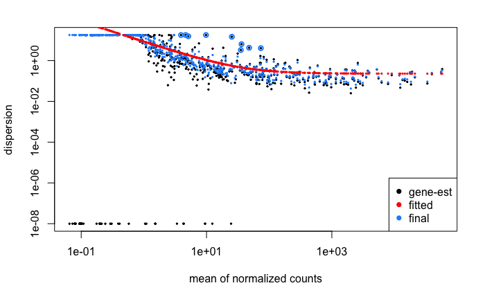
In DESeq2, an estimated gene wide mean dispersion is used to fit gene dispersions. This is important becayse RNAseq count data is heteroscedastic, lowly expressed genes have higher dispersion than highly expressed genes. Fitting gene dispersions towards the fitted line will reduce overestimation of fold changes for lowly expressed genes.
Now, lets also make a dictionary of miRNAs that have been reported to be cell type specific. This can be useful in interpreting differences differentially expressed miRNAs.
McCall, Matthew N; Kim, Min-Sik; Adil, Mohammed; Patil, Arun H; Lu, Yin; Mitchell, Christopher J; Leal-Rojas, Pamela; Xu, Jinchong; Kumar, Manoj; Dawson, Valina L; Dawson, Ted M; Baras, Alexander S; Rosenberg, Avi Z; Arking, Dan E; Burns, Kathleen H; Pandey, Akhilesh; Halushka, Marc K Toward the human cellular microRNAome Genome Res. October 2017
"
Create a dictionary of known cell specific miRNAs
"

cell_spec_dict <- list(
  "CD14+ Monocyte"   = c("Hsa-Mir-15-P1a_5p","Hsa-Mir-15-P1b_5p", "Hsa-Mir-17-P1a_5p/P1b_5p"),

  "Dendritic Cell"   = c("Hsa-Mir-146-P2_5p", "Hsa-Mir-342_3p", "Hsa-Mir-142_3p",
                         "Hsa-Mir-223_3p"),

  "Endothelial Cell" = c("Hsa-Mir-126_5p"),

  "Epithelial Cell"  = c("Hsa-Mir-8-P2a_3p", "Hsa-Mir-8-P2b_3p", "Hsa0Mir-205-P1_5p",
                        "Hsa-Mir-192-P1_5p/P2_5p", "Hsa-Mir-375_3p"),

  "Islet Cell"       = c("Hsa-Mir-375_3p", "Hsa-Mir-154-P7_5p", "Hsa-Mir-7-P1_5p/P2_5p/P3_5p"),

  "Lymphocyte"       = c("Hsa-Mir-146-P2_5p", "Hsa-Mir-342_3p", "Hsa-Mir-150_5p",
                        "Hsa-Mir-155_5p"),

  "Macrophage"       = c("Hsa-Mir-342_3p", "Hsa-Mir-142_3p", "Hsa-Mir-223_3p",
                         "Hsa-Mir-155_5p", "Hsa-Mir-24-P1_3p/P2_3p",
                         "Hsa-Mir-185_5p"),

  "Melanocyte"       = c("Hsa-Mir-185_5p", "Hsa-Mir-204-P2_5p"),

  "Mesenchymal"      = c("Hsa-Mir-185_5p", "Hsa-Mir-143_3p", "Hsa-Mir-145_5p"),

  "Neural"           = c("Hsa-Mir-375_3p", "Hsa-Mir-154-P7_5p", "Hsa-Mir-7-P1_5p/P2_5p/P3_5p",
                         "Hsa-Mir-128-P1_3p/P2_3p", "Hsa-Mir-129-P1_5p/P2_5p",
                         "Hsa-Mir-9-P1_5p/P2_5p/P3_5p","Hsa-Mir-430-P2_3p",
                         "Hsa-Mir-430-P4_3p"),

  "Platelet"         = c("Hsa-Mir-126_5p", "Hsa-Mir-486_5p"),

  "Red Blood Cell"   = c("Hsa-Mir-486_5p", "Hsa-Mir-451_5p", "Hsa-Mir-144_5p"),

  "Retinal Epithelial Cell" = c("Hsa-Mir-204-P1_5p", "Hsa-Mir-204-P2_5p", "Hsa-Mir-335_5p"),

  "Skeletal Myocyte" = c("Hsa-Mir-1-P1_3p/P2_3p", "Hsa-Mir-133-P1_3p/P2_3p/P3_3p"),

  "Stem Cell"        = c("Hsa-Mir-430-P2_3p", "Hsa-Mir-430-P4_3p", "Hsa-Mir-133-P1_3p/P2_3p/P3_3p"),

  "Hepatocyte"        = c("Hsa-Mir-122_5p")
  )

cell_spec_dict_inv <- topGO::inverseList(cell_spec_dict)
Finally, we can run the actuall differential expression analysis. Firstly we will compare normal colon to normal liver.
The first part of this code chunk consists of a set of variable definitions. The first is “column” which will decide which column in the sample_info file will be used to define the experimental design. tissue_type_A sets which tissue will be the numerator, while tissue_type_B sets which column will be the denominator. Here we will be comparing normal tissues, so norm_adj_up, norm_adj_down and pCRC_adj_up and pCRC_adj_down will be left “None”. However when we compare the tumor tissues, this is where we would specify which tissues are to be the normal background expression control.
The rest of the code chunk is the same regardless of which experiment you wish to run.
Two important lines here are the two dict_sig_mirna lines. This will store the results of this differential expression analysis in a dictionary, which will allow us to call upon them when comparing tumor tissues.
nCR vs nLi
```{R fig.height=8, fig.width=8, message=FALSE, warning=FALSE} “ Define groups to compare “ column=’type.tissue’ # Column to distinguish tissue_type_A <- ‘nLi’ # Tissue Type to be numerator tissue_type_B <- ‘nCR’ # Tissue Type to be denominator norm_adj_up = “None” # Set diffexp experiment to use as control, set None if to not do this norm_adj_down = “None” # Set diffexp experiment to use as control, set None if to not do this pCRC_adj_up = “None” # Set diffexp experiment to use as control, set None if to not do this pCRC_adj_down = “None” # Set diffexp experiment to use as control, set None if to not do this coef <- paste(column, tissue_type_A, ‘vs’, tissue_type_B, sep=’’) “ Run DiffExp experiment “ result <- (GetResults(dds, column, coef, tissue_type_A, tissue_type_B, norm_adj_up, norm_adj_down, pCRC_adj_up, pCRC_adj_down, lfc.Threshold, rpm.Threshold)) res <- result$res dict_sig_mirna[paste(coef, ‘up’, sep=’’)] <- list(res$up_mirna) dict_sig_mirna[paste(coef, ‘down’, sep=’_’)] <- list(res$down_mirna) res_res <- res$res res_dict[coef] <- res_res result$signature_mirnas$up_mirna result$signature_mirnas$down_mirna
<p align="center">
<img src="/images/volcanoplot_ncr_vs_nli" width="350" title="volcanoplot_ncr_vs_nli">
</p>


Lets also make a comparison between normal colon and normal lung. The only difference here is to specify nLu as the numerator.
## nCR vs nLu
```{R fig.height=8, fig.width=8, message=FALSE, warning=FALSE}
"
Define groups to compare
"
column='type.tissue'                 # Column to distinguish
tissue_type_A <- 'nLu'               # Tissue Type to be numerator
tissue_type_B <- 'nCR'               # Tissue Type to be denominator
norm_adj_up   = "None"               # Set diffexp experiment to use as control, set None if to not do this
norm_adj_down = "None"               # Set diffexp experiment to use as control, set None if to not do this
pCRC_adj_up   = "None"               # Set diffexp experiment to use as control, set None if to not do this
pCRC_adj_down = "None"               # Set diffexp experiment to use as control, set None if to not do this
coef <- paste(column, tissue_type_A, 'vs', tissue_type_B, sep='_')
"
Run DiffExp experiment
"
result <- (GetResults(dds, column, coef, tissue_type_A, tissue_type_B,
                       norm_adj_up, norm_adj_down,
                       pCRC_adj_up, pCRC_adj_down,
                       lfc.Threshold, rpm.Threshold))
res <- result$res
dict_sig_mirna[paste(coef, 'up', sep='_')] <- list(res$up_mirna)
dict_sig_mirna[paste(coef, 'down', sep='_')] <- list(res$down_mirna)
res_res <- res$res
res_dict[coef] <- res_res
result$signature_mirnas$up_mirna
result$signature_mirnas$down_mirna

```{R message=FALSE, warning=FALSE, cache=FALSE} ref <- ‘pCRC’ dds <- DeseqObject(design, ‘type.tissue’, countdata, sampleinfo, “None”, “None”, ref) #
It is also important to compare the primary tumor against the normal adjacent metastatic tissues. The next two code chunks are identical to the two prior, except we set pCRC in the denominator.

## pCRC vs nLi
```{R fig.height=8, fig.width=8, message=FALSE, warning=FALSE}
"
Define groups to compare
"
column='type.tissue'                 # Column to distinguish
tissue_type_A <- 'nLi'               # Tissue Type to be numerator
tissue_type_B <- 'pCRC'              # Tissue Type to be denominator
norm_adj_up   = "None"               # Set diffexp experiment to use as control, set None if to not do this
norm_adj_down = "None"               # Set diffexp experiment to use as control, set None if to not do this
pCRC_adj_up   = "None"               # Set diffexp experiment to use as control, set None if to not do this
pCRC_adj_down = "None"               # Set diffexp experiment to use as control, set None if to not do this
coef <- paste(column, tissue_type_A, 'vs', tissue_type_B, sep='_')
"
Run DiffExp experiment
"
result <- (GetResults(dds, column, coef, tissue_type_A, tissue_type_B,
                       norm_adj_up, norm_adj_down,
                       pCRC_adj_up, pCRC_adj_down,
                       lfc.Threshold, rpm.Threshold))
res <- result$res
dict_sig_mirna[paste(coef, 'up', sep='_')] <- list(res$up_mirna)
dict_sig_mirna[paste(coef, 'down', sep='_')] <- list(res$down_mirna)
res_res <- res$res
res_dict[coef] <- res_res
result$signature_mirnas$up_mirna
result$signature_mirnas$down_mirna

pCRC vs nLu
```{R fig.height=8, fig.width=8, message=FALSE, warning=FALSE} “ Define groups to compare “ column=’type.tissue’ # Column to distinguish tissue_type_A <- ‘nLu’ # Tissue Type to be numerator tissue_type_B <- ‘pCRC’ # Tissue Type to be denominator norm_adj_up = “None” # Set diffexp experiment to use as control, set None if to not do this norm_adj_down = “None” # Set diffexp experiment to use as control, set None if to not do this pCRC_adj_up = “None” # Set diffexp experiment to use as control, set None if to not do this pCRC_adj_down = “None” # Set diffexp experiment to use as control, set None if to not do this coef <- paste(column, tissue_type_A, ‘vs’, tissue_type_B, sep=’’) “ Run DiffExp experiment “ result <- (GetResults(dds, column, coef, tissue_type_A, tissue_type_B, norm_adj_up, norm_adj_down, pCRC_adj_up, pCRC_adj_down, lfc.Threshold, rpm.Threshold)) res <- result$res dict_sig_mirna[paste(coef, ‘up’, sep=’’)] <- list(res$up_mirna) dict_sig_mirna[paste(coef, ‘down’, sep=’_’)] <- list(res$down_mirna) res_res <- res$res res_dict[coef] <- res_res result$signature_mirnas$up_mirna result$signature_mirnas$down_mirna
<p align="center">
<img src="/images/volcanoplot_pcrc_vs_nlu" width="350" title="volcanoplot_pcrc_vs_nlu">
</p>

The most important function of running these experiments was to store the results in the dict_sig_mirna dictionary. This will allow us to call them during the differential expression of the tumor tissues, and avoid potential confounders due to presence of normal adjacent tissue cells!


Finally, we are ready to run the differential expression analysis between primary tumor and the metastatic sites!

The only difference this time around is that we also specify the experiments to use to control for normal background expression. If a differentially expressed miRNA is differentially expressed in the same direction in the normal background tissue, they are flagged as such in the list of differentially expressed miRNAs.

First lets run pCRC versus mLi, and use nLi vs nCR and also pCRC vs nLi, to control for normal background expression.


## pCRC vs mLi
```{R fig.height=8, fig.width=8, message=FALSE, warning=FALSE}

"
Primary tumor versus metastasis, control also with pCRC versus normal liver
"

column='type.tissue'                                           # Column to distinguish
tissue_type_A <- 'mLi'                                         # Tissue Type to be numerator
tissue_type_B <- 'pCRC'                                        # Tissue Type to be denominator
norm_adj_up   = dict_sig_mirna$type.tissue_nLi_vs_nCR_up       # Set diffexp experiment to use as control
norm_adj_down = dict_sig_mirna$type.tissue_nLi_vs_nCR_down     # Set diffexp experiment to use as control
pCRC_adj_up   = dict_sig_mirna$type.tissue_nLi_vs_pCRC_up      # Set diffexp experiment to use as control
pCRC_adj_down = dict_sig_mirna$type.tissue_nLi_vs_pCRC_down    # Set diffexp experiment to use as control
palette <- 'jco'
coef <- paste(column, tissue_type_A, 'vs', tissue_type_B, sep='_')
"
Run DiffExp experiment
"
result <- (GetResults(dds, column, coef, tissue_type_A, tissue_type_B,
                       norm_adj_up, norm_adj_down,
                       pCRC_adj_up, pCRC_adj_down,
                       lfc.Threshold, rpm.Threshold))
res <- result$res
dict_sig_mirna[paste(coef, 'up', sep='_')] <- list(res$up_mirna)
dict_sig_mirna[paste(coef, 'down', sep='_')] <- list(res$down_mirna)
res_res <- res$res
res_dict[coef] <- res_res
result$signature_mirnas$up_mirna
result$signature_mirnas$down_mirna

res_tibble <- res$res
res_tibble$miRNA <- rownames(res_tibble)
res_tibble <- as_tibble(res_tibble)

metslfc <- res_dict[[coef]]$log2FoldChange
normlfc <- res_dict[[coef]]$log2FoldChange

res_tibble$LFC_adj_background <- mapply(SubtractLFC, metslfc, normlfc)

metsP <- res_dict[[coef]]$padj
normP <- res_dict[[coef]]$padj

res_tibble$padj_subt_normal <- mapply( SubtractAdjP, metslfc, normlfc, metsP, normP )

#res_tibble %>% select(miRNA, log2FoldChange, lfcSE, LFC_adj_background, padj_subt_normal, baseMean, stat, pvalue, padj) %>% write_csv(path = '/Users/eirikhoy/Dropbox/projects/comet_analysis/data/Deseq_result_clm_vs_pcrc.csv')


Here we see four upregulated miRNAs: Hsa-Mir-204-P1_5p, Hsa-Mir-335_5p, Hsa-Mir-122_5p and Hsa-Mir-10-P2a_5p. However, all of them are also upregulated in the surounding normal tissue, thus these likely reflect the effect of normal background expression. Indeed, Mir-122_5p is specific to hepatocytes, so its apparent upregulation likely reflects the presence of some normal hepatocytes in the metastasis tissue.

Also of note, Hsa-Mir-486_5p is much lower in mLi (1336 RPM) compared to pCRC (7914 RPM). Again, when looking at the cell type specific column, we see that this miRNA is specific to platelet and red blood cells. Thus, the lower expression of this miRNA in mLi tissue may be reflective of a more hypoxic microenvironment in mLi.
Lets also run pCRC versus mLu, and use nLu vs nCR, and also nLu vs pCRC, to control for normal background expression.
pCRC vs mLu
```{R fig.height=8, fig.width=8, message=FALSE, warning=FALSE}
” Primary tumor versus metastasis, control also with pCRC versus normal liver “
column=’type.tissue’ # Column to distinguish tissue_type_A <- ‘mLu’ # Tissue Type to be numerator tissue_type_B <- ‘pCRC’ # Tissue Type to be denominator norm_adj_up = dict_sig_mirna$type.tissue_nLu_vs_nCR_up # Set diffexp experiment to use as control norm_adj_down = dict_sig_mirna$type.tissue_nLu_vs_nCR_down # Set diffexp experiment to use as control pCRC_adj_up = dict_sig_mirna$type.tissue_nLu_vs_pCRC_up # Set diffexp experiment to use as control pCRC_adj_down = dict_sig_mirna$type.tissue_nLu_vs_pCRC_down # Set diffexp experiment to use as control palette <- ‘jco’ coef <- paste(column, tissue_type_A, ‘vs’, tissue_type_B, sep=’’) “ Run DiffExp experiment “ result <- (GetResults(dds, column, coef, tissue_type_A, tissue_type_B, norm_adj_up, norm_adj_down, pCRC_adj_up, pCRC_adj_down, lfc.Threshold, rpm.Threshold)) res <- result$res dict_sig_mirna[paste(coef, ‘up’, sep=’’)] <- list(res$up_mirna) dict_sig_mirna[paste(coef, ‘down’, sep=’_’)] <- list(res$down_mirna) res_res <- res$res res_dict[coef] <- res_res result$signature_mirnas$up_mirna result$signature_mirnas$down_mirna
res_tibble <- res$res res_tibble$miRNA <- rownames(res_tibble) res_tibble <- as_tibble(res_tibble)
metslfc <- res_dict[[coef]]$log2FoldChange normlfc <- res_dict[[coef]]$log2FoldChange
res_tibble$LFC_adj_background <- mapply(SubtractLFC, metslfc, normlfc)
metsP <- res_dict[[coef]]$padj normP <- res_dict[[coef]]$padj
res_tibble$padj_subt_normal <- mapply( SubtractAdjP, metslfc, normlfc, metsP, normP )
#res_tibble %>% select(miRNA, log2FoldChange, lfcSE, LFC_adj_background, padj_subt_normal, baseMean, stat, pvalue, padj) %>% write_csv(path = ‘/Users/eirikhoy/Dropbox/projects/comet_analysis/data/Deseq_result_clm_vs_pcrc.csv’) ```

Here we see up to nine apparently upregulated miRNAs, however five of them are likely due to normal background expression. Hsa-Mir-205-P1_5p, Hsa-Mir-34-P2b_5p and Hsa-Mir-146-P1_5p, however, can not be explained as due to background expression, thus may be reflective of site specific adaptations to the new lung microenvironment. Notably, the lymphocyte specific Mir-146-P2_5p was also much higher in mLu (15251 RPM vs 1551 RPM) , possibly reflecting a higher density of lymphocytes in this new microenvironment.

Six miRNA also had lower expression in mLu, two of which likely reflect normal background expression. Furthermore the hepatocyte specific Hsa-Mir-122_5p had no reads in mLu, and again the platelet and red blood cell specific Hsa-Mir-486_5p had much lower expression levels, possibly reflecting a more hypoxic microenviornment in the metastatic lesions. Hsa-Mir-127_3p and Hsa-Mir-361_3p* also had lower expression in mLu, possibly reflecting site specific adaptations.